
R mlr3 random forest
-
date_range 20/01/2024 17:30 infosortRlabelRmachine-learningmlr3
Introduction to random forest using mlr3.
mlr3 action一下
需求:建立二分类结局的随机森林预测模型。
过程:
1.纳入全部特征,训练集上训练模型,调参,得到模型的超参数。
2.使用以上的超参数,建立包含全部特征的预测模型,得到各个特征的变量重要性。
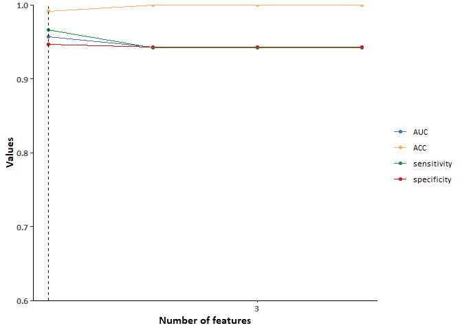
3.根据变量重要性,逐个纳入变量到随机森林模型中,并计算纳入不同数量变量时的模型评价指标。
4.选择达到合适模型评价指标时,包含最少特征的模型作为最终模型。
1
2
3
4
5
6
7
8
library(tidyverse)
library(mlr3verse)
mydat <- iris %>%
  filter(Species != "setosa") %>%
  mutate_at("Species", factor,
            levels = c("versicolor", "virginica"),
            labels = c(0,1))
knitr::kable(mydat[1:5,], digits = 3, align = 'c')
| Sepal.Length | Sepal.Width | Petal.Length | Petal.Width | Species |
|---|---|---|---|---|
| 7.0 | 3.2 | 4.7 | 1.4 | 0 |
| 6.4 | 3.2 | 4.5 | 1.5 | 0 |
| 6.9 | 3.1 | 4.9 | 1.5 | 0 |
| 5.5 | 2.3 | 4.0 | 1.3 | 0 |
| 6.5 | 2.8 | 4.6 | 1.5 | 0 |
1
2
3
4
5
6
7
8
9
10
11
12
13
14
15
16
17
18
19
20
# 设置学习器和任务
set.seed(121)
mytask = TaskClassif$new("irisStudy", mydat, target = "Species", positive = "1")
mytask$nrow
splits = partition(mytask, ratio = 0.7)

mylearner = lrn("classif.ranger", importance = "impurity",
            predict_type = "prob", seed = 121)
# 稍微调参
task_trian <- mytask$clone()$filter(rows = splits$train)
task_trian$nrow
mytune = tune(tuner = tnr("random_search"),
            task = task_trian,
            learner = lrn("classif.ranger", importance = "impurity",    seed = 121,
            predict_type = "prob", max.depth = to_tune(1, 10)),
            resampling = rsmp("repeated_cv", repeats = 10, folds = 5),
            measures = msr("classif.ce"),
            terminator = trm("evals", n_evals = 40))
mytune$archive
mytune$result_learner_param_vals
1
2
3
4
5
6
7
8
9
10
# 设置学习器参数
mylearner$param_set$values = mytune$result_learner_param_vals
# 重新训练模型
mylearner$train(mytask, row_ids = splits$train)
# 查看模型结果
mylearner$importance()
## Petal.Length  Petal.Width Sepal.Length  Sepal.Width
##   16.9508446   11.3301055    2.4145580    0.1500099
mylearner$oob_error()
## [1] 0.04483554
1
2
3
4
5
6
7
8
nvar <- length(mylearner$importance())
ooo <- matrix(FALSE, nrow = nvar , ncol = nvar)
ooo[lower.tri(ooo)] <- TRUE
diag(ooo) <- TRUE
dimnames(ooo)[[2]] <- names(mylearner$importance())
# 创建设计点
mydesign <- data.table(ooo)
knitr::kable(mydesign, digits = 3, align = 'c')
| Petal.Length | Petal.Width | Sepal.Length | Sepal.Width |
|---|---|---|---|
| TRUE | FALSE | FALSE | FALSE |
| TRUE | TRUE | FALSE | FALSE |
| TRUE | TRUE | TRUE | FALSE |
| TRUE | TRUE | TRUE | TRUE |
1
2
3
4
5
6
7
8
9
10
11
12
13
14
15
16
17
18
19
20
21
22
23
24
25
26
27
28
29
30
31
myinstance = fselect(
  fselector = fs("design_points", design = mydesign),
  task = task_trian,
  learner = mylearner,
  resampling = rsmp("cv", folds = 5),
  measures = msrs(c("classif.auc", "classif.acc",
                    "classif.sensitivity", "classif.specificity"))
)

out <- as.data.table(myinstance$archive) %>%
  select(batch_nr, features, classif.auc, classif.acc,
         classif.sensitivity, classif.specificity)
# 设置一下字体
windowsFonts(Cab = windowsFont(family = "Calibri"))
out %>%
  pivot_longer(cols = 3:6, names_to = c("task", "eval"),
               names_sep = "\\.", values_to = "value") %>%
ggplot(aes(x = batch_nr)) +
  geom_point(aes(y = value, color = eval), size = 1.4) +
  geom_line(aes(y = value, color = eval), linewidth = 0.6) +
  geom_segment(aes(x = 1, y = 0.6, xend = 1, yend = 1), linewidth=0.6,linetype="dashed") +
  theme_classic(base_family = "Cab") +
  scale_colour_manual(NULL, values = c("#4575b4","#fdae61","#1a9641","#d7191c"),
                      labels = c("AUC","ACC","sensitivity","specificity")) +
  labs(x = 'Number of features', y = 'Values') +
  scale_y_continuous(limits = c(0.6, 1), expand = c(0, 0), breaks = seq(0.6, 1, 0.1)) +
  scale_x_continuous(breaks = c(3, 5, 10, 15, 20)) +
  theme(axis.text.x = element_text(face = "bold", size =10),
        axis.title.x = element_text(face = "bold", size =12),
        axis.text.y = element_text(face = "bold",size = 10),
        axis.title.y = element_text(face = "bold",size = 12))
1
2
3
4
5
6
7
8
9
10
11
12
13
14
15
16
17
18
19
20
21
22
23
24
25
mytask$select(myinstance$result_feature_set[[1]])
mylearner$train(mytask, row_ids = splits$train)
mylearner$predict(mytask, row_ids = splits$test)

## <PredictionClassif> for 30 observations:
##     row_ids truth response      prob.1       prob.0
##           3     0        1 0.604905852 0.3950941476
##           5     0        0 0.000211427 0.9997885730
##          17     0        0 0.000211427 0.9997885730
## ---
##          92     1        1 0.995207034 0.0047929661
##          98     1        1 0.999405086 0.0005949141
##          99     1        1 0.999405086 0.0005949141

mylearner$predict(mytask, row_ids = splits$test)$score(msrs(c("classif.auc", "classif.acc",
                                                              "classif.sensitivity", "classif.specificity")))
##         classif.auc         classif.acc classif.sensitivity classif.specificity
##           0.9355556           0.8666667           0.8666667           0.8666667

mylearner$importance()
## Petal.Length
##      31.5415

mylearner$oob_error()
## [1] 0.0521194