Introduction to forest plot in R.
R 自定义森林图
1.回归结果森林图回归分析结果的森林图(forest plot),一般是在平面直角坐标系中,以一条垂直于X轴的无效线(通常坐标X=1或0)为中心,用若干条平行于X轴的线段,来表示每个变量的效应量大小及其95%可信区间。
2.生存分析1
2
3
4
5
6
7
8
9
10
11
12
13
14
15
16
17
18
19
20
21
22
23
24
25
26
27
28
29
30
31
32
33
34
35
36
library(survival)
library(forestploter)
library(tibble)
library(grid)
library(knitr)
# COX模型
cox <- coxph(Surv(futime, fustat) ~ ecog.ps + rx, ovarian)
cox_out <- data.frame(HR=summary(cox)[["coefficients"]][,2],
Lower=exp(confint(cox))[,1],
Upper=exp(confint(cox))[,2],
pvalue=summary(cox)[["coefficients"]][,5])
cox_out$HRCI <- with(cox_out, sprintf("%.3f(%.3f-%.3f)", HR, Lower, Upper))
cox_out$pvalue <- with(cox_out, sprintf("%.3f", pvalue))
cox_out <- rownames_to_column(cox_out, var = "Variable")
# AFT模型(weibull分布)
aft_wbl <- survreg(Surv(futime, fustat) ~ ecog.ps + rx,
data = ovarian, dist='weibull')
aft_wbl_out <- data.frame(HR=exp(-aft_wbl[["coefficients"]][-1]/aft_wbl[["scale"]]),
Lower=exp(-confint(aft_wbl)/aft_wbl[["scale"]])[-1,2],
Upper=exp(-confint(aft_wbl)/aft_wbl[["scale"]])[-1,1],
pvalue=summary(aft_wbl)[["table"]][-c(1,4),4])
aft_wbl_out$HRCI <- with(aft_wbl_out, sprintf("%.3f(%.3f-%.3f)", HR, Lower, Upper))
aft_wbl_out$pvalue <- with(aft_wbl_out, sprintf("%.3f", pvalue))
aft_wbl_out <- rownames_to_column(aft_wbl_out, var = "Variable")
# AFT模型(exponential分布)
aft_exp <- survreg(Surv(futime, fustat) ~ ecog.ps + rx,
data = ovarian, dist="exponential")
aft_exp_out <- data.frame(HR=exp(-aft_exp[["coefficients"]][-1]),
Lower=exp(-confint(aft_exp))[-1,2],
Upper=exp(-confint(aft_exp))[-1,1],
pvalue=summary(aft_exp)[["table"]][-1,4])
aft_exp_out$HRCI <- with(aft_exp_out, sprintf("%.3f(%.3f-%.3f)", HR, Lower, Upper))
aft_exp_out$pvalue <- with(aft_exp_out, sprintf("%.3f", pvalue))
aft_exp_out <- rownames_to_column(aft_exp_out, var = "Variable")
1
2
3
4
5
6
plot_out <- rbind(cox_out, aft_exp_out, aft_wbl_out)
plot_out$Model <- c(rep("", nrow(plot_out)))
plot_out$Model[c(1,3,5)] <- c("cox", "aft_exp", "aft_weibull")
plot_out$` ` <- paste(rep("      ", nrow(plot_out)), collapse = " ")
colnames(plot_out) <- c("Variable", "HR", "Lower", "Upper", "P value", "HR(95%CI)", "Model", "")
knitr::kable(plot_out, digits = 3, align = 'c')
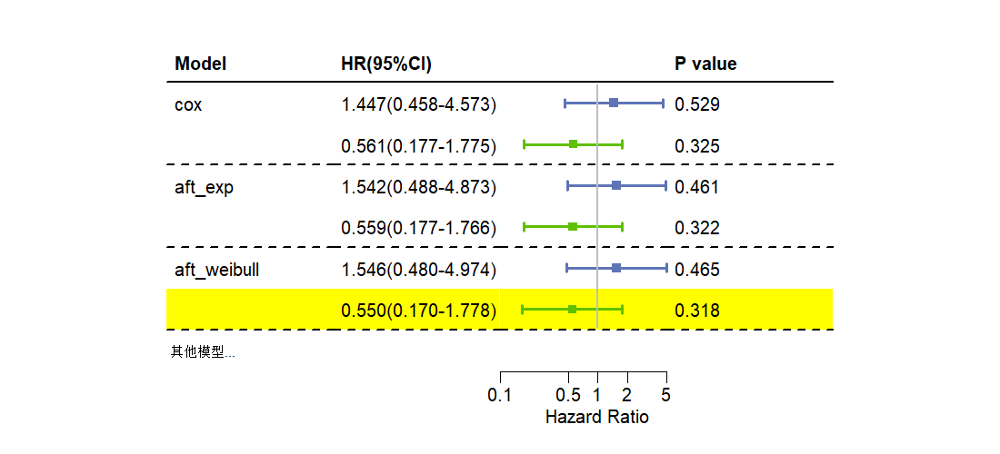
| Variable | HR | Lower | Upper | P value | HR(95%CI) | Model | |
|---|---|---|---|---|---|---|---|
| ecog.ps | 1.447 | 0.458 | 4.573 | 0.529 | 1.447(0.458-4.573) | cox | |
| rx | 0.561 | 0.177 | 1.775 | 0.325 | 0.561(0.177-1.775) | ||
| ecog.ps | 1.542 | 0.488 | 4.873 | 0.461 | 1.542(0.488-4.873) | aft_exp | |
| rx | 0.559 | 0.177 | 1.766 | 0.322 | 0.559(0.177-1.766) | ||
| ecog.ps | 1.546 | 0.480 | 4.974 | 0.465 | 1.546(0.480-4.974) | aft_weibull | |
| rx | 0.550 | 0.170 | 1.778 | 0.318 | 0.550(0.170-1.778) |
1
2
3
4
5
6
7
8
9
10
11
12
13
14
15
16
17
18
19
20
21
22
mytheme <- forest_theme(base_size = 15, ci_pch = 15, # base_family = "serif",
                        ci_alpha = 1, ci_lty = 1, ci_lwd = 3, ci_Theight = 0.2,
                        refline_lwd = 2, refline_lty = 1, refline_col = "gray",
                        xaxis_lwd = 1, xaxis_cex = 1)
plot4 <- forest(plot_out[,c(7, 6, 8, 5)],
                est = plot_out$HR, lower = plot_out$Lower, upper = plot_out$Upper,
                sizes = 0.8, ci_column = 3, ref_line = 1,
                xlab = c("Hazard Ratio"),
                x_trans = "log2",
                xlim = c(0.1, 5),
                ticks_at = c(0.1, 0.5, 1, 2, 5),
                theme = mytheme) |>
  edit_plot(which = "background", gp = gpar(fill = "white")) |>
  add_border(row = 1, part = "header", gp = gpar(lwd = 2, lty = 1), where = "bottom") |>
  add_border(row = c(2, 4, 6), part = "body", gp = gpar(lwd = 2, lty = 2), where = "bottom") |>
  edit_plot(row=c(1, 3, 5),col=3,which="ci",gp=gpar(col="#5E74B5",fill="#5E74B5")) |>
  edit_plot(row=c(2, 4, 6),col=3,which="ci",gp=gpar(col="#5FC000",fill="#5FC000")) |>
  add_border(part = "header", gp = gpar(lwd = 2, lty = 2)) |>
  edit_plot(row = 6, which = "background", gp = gpar(fill = "yellow")) |>
  insert_text(text = "其他模型...", row = 7, col = 1:4, part = "body", just = "left")

plot(plot4, autofit = TRUE)